Pool impact and two-venue cost assumptions
Separate pool curvature, fees, slippage tolerance, transfer losses and capital when examining a supplied swap or arbitrage scenario.
Start with the supported pool
Output = output reserve × effective input / (input reserve + effective input)The swap calculator supports a single full-range constant-product pool with the fee retained in its input reserve. Effective input is reduced by the fee for quoting output, while the entire input joins the reserve afterward. Hypothetical reserves of 1,000 each and an input of 100 without fees produce about 90.9091 output units. Concentrated liquidity, stable-swap curves, multi-hop routes and transfer-tax tokens require other models.
Two different shortfalls
Curve impact compares the rate for effective input with the pre-swap marginal rate. Total shortfall also includes the input fee. Minimum output applies your supplied tolerance to the modeled quote; a 1% tolerance gives 90 in the fee-free example. It is a protective bound relative to that quote, not a prediction of the eventual transaction or a guarantee of execution.
A displayed spread can disappear
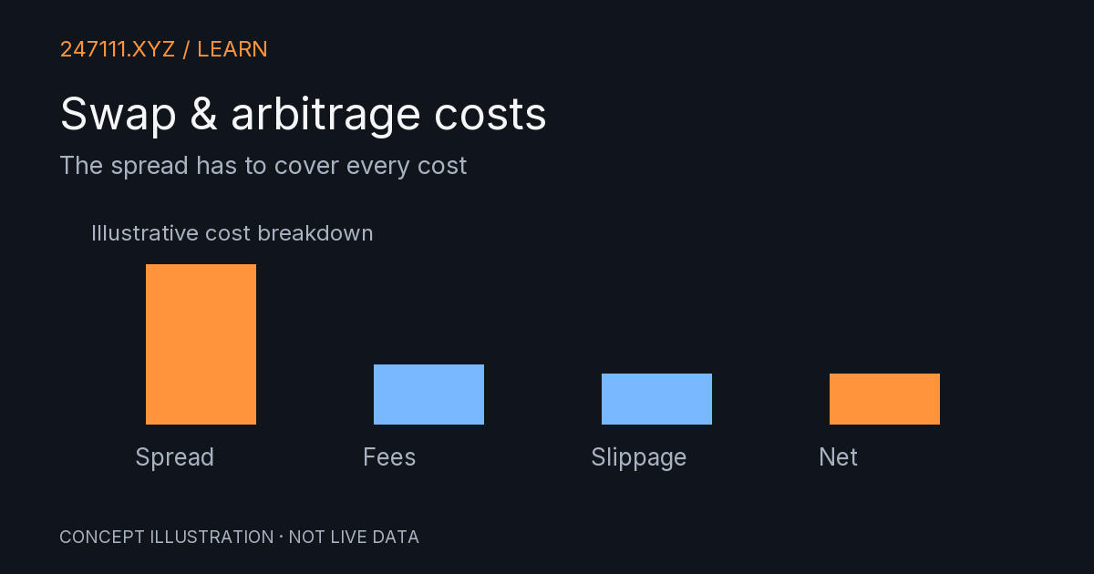
Net = fee-adjusted sale proceeds − acquisition cost − allocated quote costsThe arbitrage page starts from the supplied ask at venue A and bid at venue B. Adverse slippage changes each price, then each venue fee applies to its own side. In transfer mode the withheld token fee reduces what reaches the sale. Buying 10 at 100 with 1% buy fees costs 1,010. Selling nine at 105 after a 1% sell fee returns 935.55, leaving a 74.45 loss before any other costs.
Account for available inventory
Prefunded mode assumes sale inventory already exists at venue B; it ignores transfer fields and marks that inventory at the effective acquisition ask for the combined-capital calculation. With the same prices and fees, selling all ten gives a net 29.50 on modeled capital of 2,010. Break-even bid includes fees, losses and adverse sell slippage. A 100% sale fee leaves no finite break-even. Latency, borrowing, rebalancing, order depth and execution remain outside this scenario.